Understanding Diffusion Models as a SDE
As I’m learning diffusion models, I found these two blogs (Song & Lil’Log) help me a lot in addition to the original papers, from which this blog takes a huge reference as well. However, I find there are a little bit more details that can be discussed, especially on building the connection between DDPM and the corersponding SDE. Therefore I write this blog on top of the papers to help people learn DDPM beyond just adding noise and denoising.
Also, I’m giving a detailed 1D mixture of Gaussian example as a toy example to build more intuitives, and visualize the diffusion process. With that we can also unveil some details analytically, and discuss the controlability of diffusion models.
In this blog, we focus on summarizing the connect between the classical diffusion model (DDPM) and the score matching / stochastic differential equation (SDE). We’ll shortly describe each component separately in a high level (this may need some prior knowledge to both sides) Then we would introduce the connections in between. It would be much easier to understand (perhaps more helpful as well) if you pick up some basic knowledge on DDPM/score matching before.
DDPM, score matching & SDE
Diffusion models are first proposed as a generative model
Diffusion Model (DDPM)
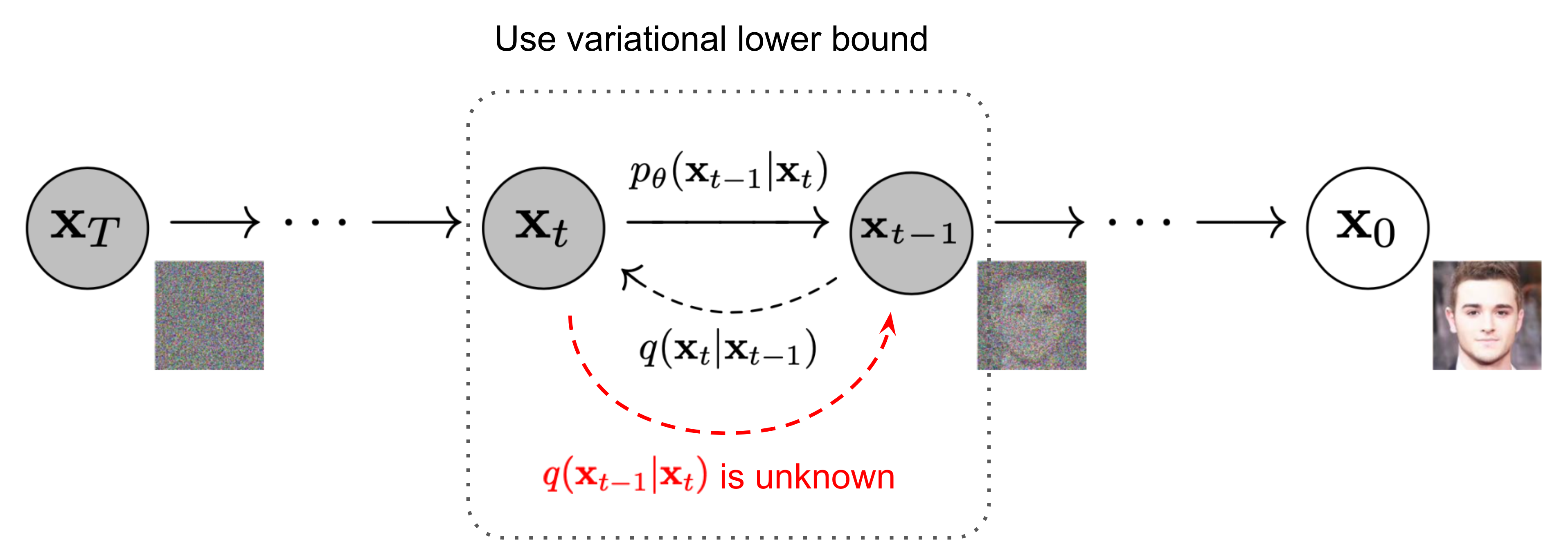
The diffusion process is defined by iteratively adding Gaussian noises into the original data, where \(p(\mathbf{x}_{t+1}\mid\mathbf{x}_t) = \mathcal{N}(\mathbf{x}_{t+1}; \sqrt{(1-\beta_t)} \mathbf{x}_t, \beta_t \mathbf{I})\), or as Eq.\eqref{eq: ddpm_pxt1x}. $\beta_t$ is a (designed) noise schedule. \(\epsilon \sim \mathcal{N}(\mathbf{0}, \mathbf{I})\). Typically, \(\beta_t\) is a linear function between, for example, \(\beta_{min}=0.001\), and \(\beta_{max}=0.02\).
Applying a reparameterization trick, we can obtain the distribution over time as Eq. \eqref{eq: ddpm_pdf}. Note that we define \(\alpha_t = 1-\beta_t\), \(\bar{\alpha}_t = \prod_{i=0}^t \alpha_i\).
\[\begin{equation} \label{eq: ddpm_pdf} p(\mathbf{x}_t\mid\mathbf{x}_0) = \mathcal{N}(\sqrt{\bar{\alpha}_t} \mathbf{x}_0, (1-\bar{\alpha}_t)\mathbf{I}) \end{equation}\]
In the sampling time, we reverse the diffusion process by iteratively denoise with a parameterized (trained) probability \(p_\theta(\mathbf{x}_{t-1}\mid\mathbf{x}_t)=\mathcal{N}(\mathbf{x}_{t-1}; \mathbf{\mu}_\theta, \mathbf{\Sigma}_\theta \mathbf{I})\). We sample \(\mathbf{x}_t\) from a zero-mean Gaussian \(\mathcal{N}(\mathbf{0}, \mathbf{I})\), and denoise in a Markov Chain with such Gaussian noise until we get \(\mathbf{x}_0\).
Score Matching
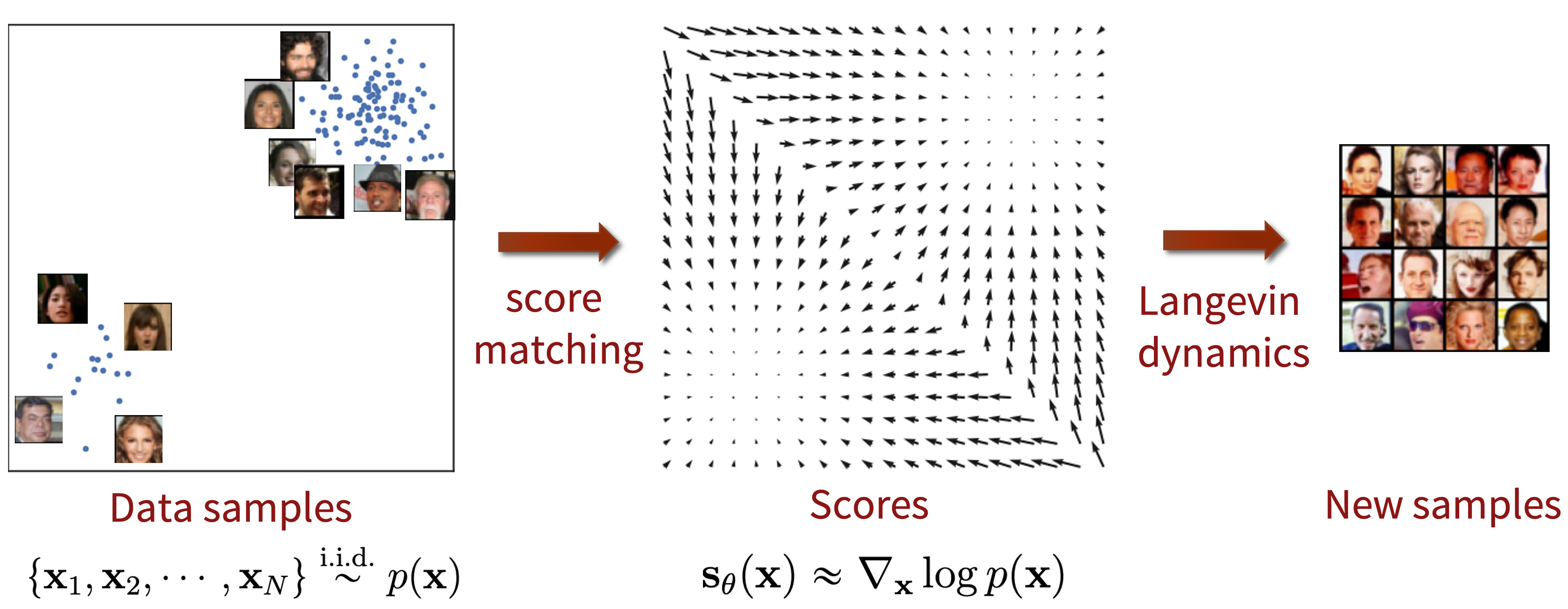
The diffusion process can be also viewed as a score matching process, where a score function is defined as the \(\nabla_\mathbf{x} \log p(\mathbf{x})\). Score function describe the gradient towar\mathrm{d}s the high probability area in the manifold. We can learn this function with a neural network \(s_\theta (\mathbf{x})\) by minimizing the fisher divergence \(\mathbb{D}_F = \mathbb{E}_{x \sim p_{data}(\mathbf{x})}\|\nabla_\mathbf{x} \log p_{data}(\mathbf{x}) - s_\theta (\mathbf{x}) \|^2_2\).

The sampling process, in this context, is formulated as a Markov Chain Monte Carlo (MCMC) process based on the Langevin dynamics, which is a concept from physics used for statistically modeling the molecular system. The sampling process is defined as Eq.\eqref{eq: smld}, with a step size \(\delta\) and a Gaussian noise \(\epsilon_t \sim \mathcal{N}(\mathbf{0}, \mathbf{I})\).
\[\begin{equation} \label{eq: smld} \mathbf{x}_{t+1} = \mathbf{x}_t + \delta \nabla_\mathbf{x} \log p(\mathbf{x}) + \sqrt{2\delta} \epsilon_t \end{equation}\]Stochastic Differentiable Equation (SDE)
Both DDPM and score matching can be formulated into a unified stocastic differentiable equation (SDE) framework, where the (reverse) diffusion process are generalized as a continuous process. A general form of a SDE is usually written as \(\mathrm{d}\mathbf{x} = f(\mathbf{x},t)\mathrm{d}t + g(\mathbf{x},t)\mathrm{d}w\). \(f(\mathbf{x},t)\) is the shifting term, and \(\mathrm{d}w\) is a random noise.
In the diffusion model context, this SDE can be designed different to describe different diffusion method. For example, in score matching perspective, an simplest example can be \(\mathrm{d}\mathbf{x} = e^t \mathrm{d}w\). This is same as perturbing the data with \(\mathcal{N}(\mathbf{0}, \sigma_1^2 \mathbf{I}), \mathcal{N}(\mathbf{0}, \sigma_2^2 \mathbf{I}), \ldots, \mathcal{N}(\mathbf{0}, \sigma_t^2 \mathbf{I})\), i.e., a sequence of zero-mean Gaussians with exponential growing variance. Or, it can be designed as the DDPM algorithm, which describe the SDE process as Eq.\eqref{eq: ddpm_as_sde}.
\[\begin{equation} \label{eq: ddpm_as_sde} \mathrm{d}\mathbf{x} = -\frac{1}{2} \beta(t) \mathbf{x} \mathrm{d}t + \sqrt{\beta(t)} \mathrm{d}w \end{equation}\]Any SDE has a corresponding reverse SDE as Eq.\eqref{eq: general_reverse_sde}, in which \(\mathrm{d}t\) is a negative infinitesimal time step, and the score function can be learnt by \(s_\theta (\mathbf{x})\).
\[\begin{equation} \label{eq: general_reverse_sde} \mathrm{d}\mathbf{x} = \left[ f(\mathbf{x}, t) - g^2(t) \nabla_\mathbf{x} \log p_t(\mathbf{x}) \right] \mathrm{d}t + g(t) \mathrm{d}w \end{equation}\]In practice, we can use Euler-Maruyama method to solve the SDE in a descritized way.
\[\label{eq: euler-maruyama} \begin{aligned} \Delta \mathbf{x} &\leftarrow \left[ f(\mathbf{x}, t) - g^2(t) \nabla_\mathbf{x} \log p_t(\mathbf{x}) \right] \mathrm{d}t + g(t) \sqrt{\mid\Delta t\mid} \epsilon \\ \mathbf{x} &\leftarrow \mathbf{x} + \Delta \mathbf{x} \\ t &\leftarrow t + \Delta t \end{aligned}\]The marginal probability density function can be calculated by solving the SDE. In the DDPM algorithm, more specifically, the corresponding ordinary differentiable equation (ODE) can be computed as below.
\[\begin{aligned} \mathrm{d}\mathbf{x} &= -\frac{1}{2} \beta_t \mathbf{x} \mathrm{d}t & \text{(math)} \\ \int_{\mathbf{x}_0}^{\mathbf{x}_t} \frac{1}{x} \mathrm{d}\mathbf{x} &= \int_0^t -\frac{1}{2} \beta_s \mathrm{d}s & \text{(integral)} \\ \log \frac{\mathbf{x}_t}{\mathbf{x}_0} &= \int_0^t -\frac{1}{2} \beta_s \mathrm{d}s & \text{(integral)} \\ \mathbf{x}_t &= e^{-\frac{1}{2} \int_0^t \beta_s \mathrm{d}s} \mathbf{x}_0 & \text{(exponential)} \end{aligned}\]The calculation of the variance of the marginal PDF can be found from
DDPM as a SDE
So far we’ve introduced the basic concept of DDPM, score matching, and diffusion as a SDE. In this section, we show they are equivalent in the following perspectives.
Gaussian Kernel
In the DDPM, we add a Gaussian noise with a noise schedule as Eq.\eqref{eq: ddpm_pxt1x}. Here we show this is consistent with the SDE formulation in Eq.\eqref{eq: ddpm_as_sde}.
Note that in this specific section, we need to differentiate the noise we use in SDE, denoted by \(\beta(t)\), and the noise from original DDPM \(\beta_t\). They have a scale relationship in between, \(\beta_t = \beta(t) \Delta t\) so that they contribute equally when applying the integral.
\[\begin{aligned} \mathbf{x}_{t+1} &= \sqrt{(1-\beta_t)} \mathbf{x}_t + \sqrt{\beta_t} \epsilon & \text{(DDPM)} \\ \mathbf{x}(t+\Delta t) &= \sqrt{(1-\beta(t)\Delta t)} \mathbf{x}(t) + \sqrt{\beta(t) \Delta t} \epsilon & \text{(discrete to continuous)} \\ \mathbf{x}(t+\Delta t) &= (1 + \frac{1}{2}\frac{-\beta(t)\Delta t}{\sqrt{(1-\beta(t)\Delta t)}}) \mathbf{x}(t) + \sqrt{\beta(t) \Delta t} \epsilon & \text{(Taylor Expansion)} \\ \mathbf{x}(t+\Delta t) &= (1 + \frac{1}{2}\frac{-\beta(t)\Delta t}{1}) \mathbf{x}(t) + \sqrt{\beta(t) \Delta t} \epsilon & (\beta(t)\Delta t << 1) \\ \mathbf{x}(t+\Delta t) - \mathbf{x}(t) &= - \frac{1}{2}\beta(t)\Delta t \mathbf{x}(t) + \sqrt{\beta(t) \Delta t} \epsilon & \text{(re-write)} \\ \mathrm{d}\mathbf{x} &= - \frac{1}{2}\beta(t) \mathbf{x}(t) \mathrm{d}t + \sqrt{\beta(t)} \mathrm{d}w & \text{(VP SDE)} \end{aligned}\]This way we show that the Gaussian kernel applied to the DDPM process is equiavalent to the variance preserving (VP) SDE defined in
Probability Density Function
We can also compare the probability density function from both DDPM and SDE perspectives. In DDPM, we describe the PDF as \(p(\mathbf{x}_t \mid \mathbf{x}_0) = \mathcal{N}(\mathbf{x}_t; \sqrt{\bar{\alpha_t}} \mathbf{x}_t, (1-\bar{\alpha_t})\mathbf{I})\) in Eq.~\eqref{eq: ddpm_pdf}. In SDE, we previously show \(p(\mathbf{x}(t) \mid \mathbf{x}(0)) = \mathcal{N}(\mathbf{x}(t); e^{-\frac{1}{2} \int_0^t \beta(s) \mathrm{d}s} \mathbf{x}(0), [1 - e^{-\int_0^t \beta(s) \mathrm{d}s}] \mathbf{I})\) in Eq.\eqref{eq: ddpm_sde_pdf}.
Here we’ll first show that \(\sqrt{\bar{\alpha_t}}\) is a good approximation of \(e^{-\frac{1}{2} \int_0^t \beta(s) \mathrm{d}s}\). Again, \(\beta_t = \beta(t) \Delta t\).
\[\begin{aligned} \ln(1-\beta_i) &\simeq -\beta_i & (\beta_i \ll 1, \ln x \simeq (x-1) \text{ when } x \simeq 1) \\ \ln \prod_{i=1}^t (1-\beta_i) &\simeq -\sum_{i=1}^t \beta_i & (\text{logarithm}) \\ \prod_{i=1}^t (1-\beta_i) &\simeq \exp \left( -\sum_{i=1}^t \beta_i \right) & (\text{exponentiating}) \\ \bar{\alpha_t} &\simeq \exp \left( -\sum_{i=1}^t \beta_i \right) & (\text{definition}) \\ \sqrt{\bar{\alpha_t}} &\simeq \exp \left( -\frac{1}{2} \sum_{i=1}^t \beta_i \right) & (\text{square root}) \\ \sqrt{\bar{\alpha_t}} &\simeq \exp \left( -\frac{1}{2} \int_0^t \beta(s) \mathrm{d}s \right) & (\text{Riemann sum}) \end{aligned}\]For the variance, we have
\[\begin{aligned} \sqrt{\bar{\alpha_t}} &\simeq \exp \left( -\frac{1}{2} \int_0^t \beta(s) \mathrm{d}s \right) & \\ \bar{\alpha_t} &\simeq \left( \exp (-\frac{1}{2} \int_0^t \beta(s) \mathrm{d}s ) \right)^2 & (\text{square}) \\ 1 - \bar{\alpha_t} &\simeq 1 - e^{-\int_0^t \beta_s \mathrm{d}s} & (\text{math}) \end{aligned}\]Reverse Process
The DDPM reverse process is defined by
\[\begin{equation} \label{eq: ddpm_denoise} \begin{split} \mathbf{x}_{t-1} = \frac{1}{\sqrt{\alpha_t}} (\mathbf{x}_t - \frac{\beta_t}{\sqrt{1 - \bar{\alpha_t}}} \epsilon_\theta(\mathbf{x}_t, t, \mathbf{c})) + \sqrt{\bar{\beta_t}} \epsilon \\ \end{split} \end{equation}\]Where the reverse SDE process for DDPM can be written as \refeq{eq: ddpm_reverse_sde}
\[\begin{equation} \label{eq: ddpm_reverse_sde} \begin{split} \mathrm{d}\mathbf{x} &= \left[ f(\mathbf{x}, t) - g^2(t) \nabla_\mathbf{x} \log p_t(\mathbf{x}) \right] \mathrm{d}t + g(t) \mathrm{d}w \\ &= \left[ -\frac{1}{2} \beta(t) \mathbf{x} - \beta(t) \nabla_\mathbf{x} \log p_t(\mathbf{x}) \right] \mathrm{d}t + \sqrt{\beta_t} \mathrm{d}w \end{split} \end{equation}\]Example: 1D Mixture of Gaussian
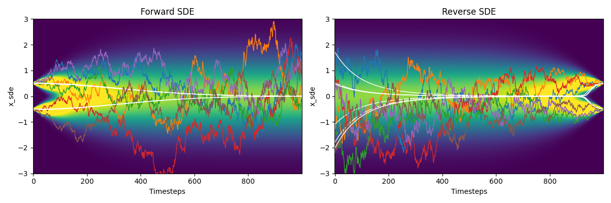
Let’s consider a 1D diffusion process so that we have a more direct intuitive, also we have some analytical result. Define the data distribution we are interested in as a mixture of Gaussian (MoG), \(p(x_0) = \sum_{i=\{1, 2\}} \pi_i \mathcal{N}(\mu_i, \sigma_i^2)\).
Notably, since we have the original data distribution, we can obtain the marginal probability density function $p(x_t)$ in the diffusion process. It will be another Gaussian, which we can compute the mean and the variance separately. For a single Gaussian component, denote \(p(x_t\mid x_0) = \mathcal{N}(x_t; \sqrt{\bar{\alpha}_t}x_0, \sigma^2_t)\), where \(\bar{\alpha}_t = e^{-\int_0^t \beta_s \mathrm{d}s}\), \(\sigma_t = \sqrt{1 - \alpha_t}\)
Since we have the analytical solution to this probability density function, we can write the score function as well.
\[\begin{equation} \label{eq: mog_sf} \begin{split} \nabla_x \log p(x_t) &= \nabla_x \log \sum_{i=\{1, 2\}} \pi_i \mathcal{N}\left( x_t; \sqrt{\bar{\alpha}_t} \mu_i, \sigma^2_t + \bar{\alpha}_t \sigma^2_i \right) \\ &= \nabla_x \log \sum_{i=\{1, 2\}} \pi_i \frac{1}{\sqrt{2\pi (\sigma^2_t + \bar{\alpha}_t \sigma^2_i)}} \exp \left( -\frac{(x_t - \sqrt{\bar{\alpha}_t} \mu_i)^2}{2 (\sigma^2_t + \bar{\alpha}_t \sigma^2_i)} \right) \\ &= \frac{\sum_{i=\{1, 2\}} \pi_i \frac{1}{\sqrt{2\pi (\sigma^2_t + \bar{\alpha}_t \sigma^2_i)}} \exp \left( -\frac{(x_t - \sqrt{\bar{\alpha}_t} \mu_i)^2}{2 (\sigma^2_t + \bar{\alpha}_t \sigma^2_i)} \right) \left( -\frac{(x_t - \sqrt{\bar{\alpha}_t} \mu_i)}{(\sigma^2_t + \bar{\alpha}_t \sigma^2_i)} \right)}{p(x_t)} \\ &= \sum_{i=\{1, 2\}} \frac{\pi_i \mathcal{N}\left( x_t; \sqrt{\bar{\alpha}_t} \mu_i, \sigma^2_t + \bar{\alpha}_t \sigma^2_i \right)}{p(x_t)} \left( -\frac{(x_t - \sqrt{\bar{\alpha}_t} \mu_i)}{(\sigma^2_t + \bar{\alpha}_t \sigma^2_i)} \right) \\ &= \sum_{i=\{1, 2\}} \gamma_i \left( -\frac{(x_t - \sqrt{\bar{\alpha}_t} \mu_i)}{(\sigma^2_t + \bar{\alpha}_t \sigma^2_i)} \right) \end{split} \end{equation}\]where \(\gamma_i = \frac{\pi_i \mathcal{N}\left( x_t; \sqrt{\bar{\alpha}_t} \mu_i, \sigma^2_t + \bar{\alpha}_t \sigma^2_i \right)}{p(x_t)}\) is the probability portion (weight) for a Gaussian component.
If we use a linear noise schedule, \(\beta_t = \beta_{min} + t (\beta_{max} - \beta{min})\), we can either obtain the close-form solution for \(\bar{\alpha}_t = e^{-(\frac{1}{2}t^2(\beta_{max} - \beta_{min}) + t \beta_{min})}\), or use Riemann approximation \(\bar{\alpha}_t = e^{-\sum(\beta_t \Delta t)}\) (more generalized method).
We visualize this analytical solution as the figure below.

Conditioned Generation
One advantage of diffusion model is its controlability using the conditioned diffusion generation process. It was originally described as the perturbed gaussian transition in
Considering the following joint probability \(p(\mathbf{x}, y)\), where \(y\) can be a label/caption to an image. Applying the Bayesian rule, we have
\[\begin{equation} \label{eq: sm_joint_prob} \begin{split} p(\mathbf{x}_t, y) &= p(\mathbf{x}_t) p(y\mid\mathbf{x}_t) \\ \nabla_{\mathbf{x}} \log p(\mathbf{x}_t, y) &= \nabla_{\mathbf{x}} \log p(\mathbf{x}_t) + \nabla_{\mathbf{x}} \log p(y\mid\mathbf{x}_t) \\ \end{split} \end{equation}\]If we have an explicit classifier \(p(y \mid \mathbf{x}) = f_\phi(y \mid \mathbf{x}_t, t)\), in the DDPM context, we can use the gradient to guide the diffusion sampling process.
\[\begin{equation*} \begin{split} \nabla_{\mathbf{x}} \log p(\mathbf{x}_t, y) &= \nabla_{\mathbf{x}} \log p(\mathbf{x}_t) + \nabla_{\mathbf{x}} \log p(y\mid\mathbf{x}_t) \\ &= \nabla_{\mathbf{x}} \log p(\mathbf{x}_t) + \nabla_{\mathbf{x}} \log f_\phi(y\mid\mathbf{x}_t, t) \\ \end{split} \end{equation*}\]Guided 1D MoG Diffusion
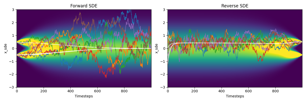
In our 1D MoG example, if we use \(p(y \mid x) = \mathcal{N}(\mu_i; \sigma^2_i)\) as our guidance, we are leading our denoising into one of the Gaussian component.
\[\begin{equation*} \nabla_{x} \log p(y \mid x_t) = \nabla_{x} \log \mathcal{N}(\mu_i; \sigma^2_i) = - \frac{x-\mu_i}{\sigma^2_i} \end{equation*}\] \[\begin{equation*} \begin{split} \nabla_{x} \log p(x_t, y) &= \nabla_{x} \log p(x_t) + \nabla_{x} \log p(y\mid x_t) \\ &= \sum_{i=\{1, 2\}} \gamma_i \left( -\frac{(x_t - \sqrt{\bar{\alpha}_t} \mu_i)}{(\sigma^2_t + \bar{\alpha}_t \sigma^2_i)} \right) - \frac{x-\mu_i}{\sigma^2_i} \end{split} \end{equation*}\]This way, as shown in the visualization below, all the samples are guided into one of the Gaussian components in the reverse SDE process.
